
Linear programming (LP)
Linear programming technique is being used in production and service management. It is the technique of choosing the best possible alternative among the various alternatives available to produce goods and services, to transport the goods produced etc. this technique may be sometimes complex because different alternatives consists of a large number of variables, giving different results.
Thus linear programming is a mathematical technique for allotting limited resources in an optimum manner. Hence, it is of great practical significance for the management for achieving the prime objective of the business, i.e. maximization of profits and minimization of cost. It is an undisputable fact that resources of a business are limited setting limit or restriction on the smooth functioning of the business. The problem confronting the management is to decide the manner in which these limited resources are to be earmarked for various’ uses so as to have the maximum profit. Linear programming is a planning technique that permits some objective functions to be minimized or maximized within the framework of given situational restrictions.
Applications of linear programming
The linear programming technique may be fruitfully applied in the following spheres:
(i) The linear programming can be used in production scheduling and inventory control so as to produce the maximum out of the resources available to satisfy the needs of the public by minimizing the cost of production and the cost of inventory control.
(ii) The technique of linear programming can also be fruitfully used in solving the blending problems. Where basic components are combined to produce a product that has certain set of specifications and one may calculate the best possible combination of these compounds which maximize the profits or minimize the costs.
(iii) Other important applications of linear programming can be in purchasing, routing, assignment and other problems having selection problems such as
(a) selecting the location of plant,
(b) deciding transportation route within the organization,
(c) utilizing the go downs and other distribution centers to the maximizing,
(d) preparing low-cost production schedules,
(e) determining the most profitable product-mix, and
(f) analyzing the effects of changes in purchase prices and sale prices.
Formulation of an LP Problem (LPP): In formulating the linear programming problem, the basic step is to set up some mathematical model. For this purpose, the following considerations should be kept in mind: (i) unknown variables, (ii) objectives and (iii) constraints. This can be done with the help of the following terms:
- The objective function: An objective function is some sort of mathematical relationship between variables under consideration. Under linear programming this relationship is always linear. The construction of objective function mainly depends upon abstraction. It is a process whereby the most important features of a system are considered.
The objective function is always positive. The coefficients &v a2are certain constants and are known as prices associated to the variables Xv X2.
- Constraints on the variables of the objective function: In practice, the objective function is to be optimized under certain restraints imposed on die variables or some combination of few or all the variables occurring in the objective function. These restrictions, in most of the cases, are never exact. Had these been exact, the objective function would have been easily optimized by die use of differential calculus. The restraints should be known and expressed in terms of linear algebraic expression.
- Feasible solution: One of the essential features of linear programming problem is optimization of linear objective function Z. It is subject to the linear constraints on the variables of the objective function. A set of values of Xv X2………which satisfies the constraints and the non- negativity restrictions are called feasible solution. A feasible solution which optimizes the objective function is known as optimal solution. Thus, a linear programming problem can be formulated in this way. There are number of ways of finding the optimal solution for a given linear programming problems. The following three methods are mainly used for this purpose.
(1) Graphic Method (2) Simplex Method (3) Transportation Method.
SIMPLEX METHOD OF LINEAR PROGRAMMING
This is the most powerful and popular method for solving linear programming problems. Any problem can be solved by this method which satisfies the conditions of linearity and certainty irrespective of the number of variables. It is an iterative procedure which ultimately gives the optimal solution.
Simplex method of linear programming is a very important technique to solve the various linear problems. Under this method, algebraic procedure is used to solve any problem which satisfies the test of linearity and certainty. It is an iterative procedure which ultimately gives the optimal solution. Several variables can be used under this method. However, the simplex method is more complex and involves somewhat unsophisticated complex mathematics.
Features:
There are two characteristic features of the simplex method which we can cite them at the very outset. First, we have the computational routine in the iterative process. Iteration means the repetition. Therefore, in working towards the optimal solution, the computational routine if repeated again and again, following a standard pattern, successive solutions are developed in a systematic pattern until the best solution is arrived. Secondly, such new solution will give a profit larger than the previous solution. This important characteristic assures us that we are always moving closer to the optimal solution.
There are two types of linear programming problems to be solved by this method:-
(1) Maximization of objective function, and (2) Minimization of objective function.
SLACK AND ARTIFICIAL VARIABLES
Slack variables:
A slack variable represents costless process whose function is to ‘use up otherwise unemployed capacity, say, machine hour or warehouse capacity. Effectually the slack variable represents unused capacity and it will be zero only, if production facilities are fully utilized. It is always non-negative or positive and explains the unallocated portion of the given limited resources. The main purpose of introducing slack variables in the simplex method of linear programming is to convert the inequalities (i.e., constraints); into equalities or, say, equations.
Artificial variables:
The artificial variables are fictitious and do not have any physical meaning. These variables are assigned a very large per unit penalty in the objective function. The penalty is designated as –M for maximization problem and +M in minimization problem where M is always greater than zero. There may be situations where the constraints involve mixture of ≥ = and ≤ signs. In such cases, the slack variables cannot provide a starting feasible solution and we have to introduce both slack and artificial variables to have a starting basis. The artificial variables are denoted as A1, A2………….An in the programme column of initial simplex tableau. These artificial variables should be removed first by using simplex criterion. If at any stage of simplex procedure the basic feasible solution contains artificial variable but the variable to be deleted at that stage is not the artificial variable, it means we are departing from the simplex criterion for selecting the variable.
The iterative procedure does not work under following circumstances –
(i) One or more artificial variables appeals in the program column at a stage when the base row values are all positive.
(ii) No artificial variables remain in the programme column.
(iii) The problem is redundant if one or more artificial variables occur in programme column and the corresponding values in the constant column are zero at a stage when all Zj-Cj are positive or non-negative.
Problem: Find the maximum value of Z = 3X1+ 5X2 + 4X3. Where X1, X2, X3 ≥ 0 subject lo the following constraints.
2X1 + 3X2 ≤ 18
2X2 + 5X3 ≤ 18
3X1 + 2X2 + 4X3 ≤ 25
Solution:
As here the objective function is to be maximised, we shall introduce the slack variables in the constraints and the objective function and we get the following equations:
2X1 + 3X2 + S1 + 0.S2 + 0.S3 = 18
2X2 + 5X3 + 0.S1 + S2 + 0.S3 = 18
3Xt + 2X2 +4X3 + 0.S1 + 0.S2 S3 = 25
So, Z = 3X1+ 5X2 + 4X3 +0S1+ 0S2 + 0S2
Now, various simplex tableaus are prepared to get the optimal solution.
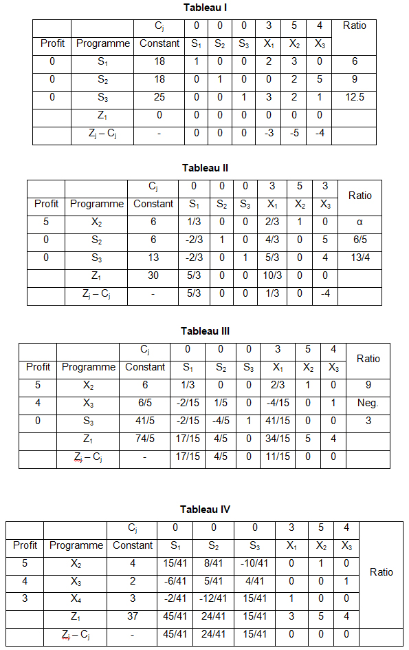
In tableau IV all Zj – Cj are non negative or positive hence it is the optimal solution. The optimal solution is X1 = 3; X2 = 4; X3 = 2 and the maximum profit Zj = 37